Bayesian Multinomial Models: A Tragedy (In Runescape)
- Abandon all hope, ye who enter
- Combat in Runescape
- The Data
- Model Criteria
- Constructing A Bayesian Model
- Using The Bayesian Model
- Conclusion: This Model Sucks
Abandon all hope, ye who enter
Originally I set out in this project to design an interesting Bayesian model which could predict opponent behavior in player-vs-player Old School Runescape combat.
I will spoil the outcome for you now. After a long and arduous journey, I discovered that my derived model absolutely blows.
It’s fascinating, really. Theoretically deriving this model was hard. It took me a very long time. I had to solve some tough integrals. And yet, the model that pops out is so disappointingly simple.
In retrospect, I could have easily guessed what the model will be without any derivations. I could have implemented the model in two lines of code.
So if the model sucks, why release this article at all? Why not bury it and move on with my life? I have a few rationalizations about this:
- This article may provoke some insights about model design. How do you design a problem so that Bayesian modeling is a good solution? Certainly not like this.
- If anyone ever wonders about the process of deriving a multinomial Bayesian model, this article contains the derivations for the case of $k=3$ possible outcomes.
- This article is proof to myself that I can do Bayesian things.
- Because it’s pretty funny, honestly.
So consider yourself warned. You may find interesting Bayesian statistics here, but you will not find a good Runescape PvP model.
Combat in Runescape
Player Vs Player (PVP) combat in Old School Runescape (OSRS) can be modeled as an iterative guessing game. At each step of the game, each player must choose two things:
- Which attack style to use
- Which attack style to defend or “pray” against
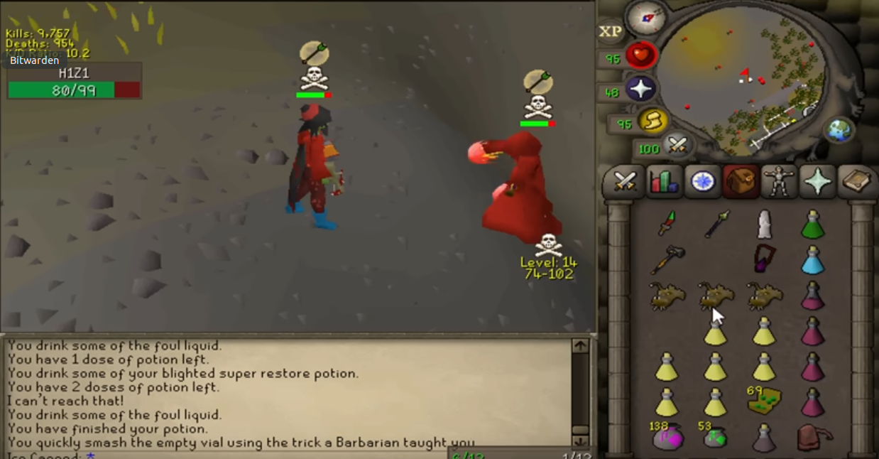
There are three attack styles in the game: Melee, Range, and Mage, each depicted with their own respective icon:


During each turn, the players attack and deal a random amount of damage. Players take less damage if they are “praying against” their opponent’s attack style.
 |
|---|
| The “overhead prayers” show both players are praying against Range. The player on the left is attacking with Range (a crossbow), while the player on the right is using Mage. Consequently, the player on the right will take reduced damage, while the player on the left will take the normal amount of damage. |
Thus, it is very important to attempt to predict your opponent’s behavior (informally called “reading”) in order pray against the correct attacks and attack with an off-prayer style. As seen in this video, professional players like Odablock are extremely skilled at reading their opponents:
Actual Runescape combat is more elaborate than the iterative guessing game concept we described above. Rather than being truly iterative, actions occur within the tick system of the Runescape clock where different weapons have different speeds. There are also more actions than simply attacking, such as eating or drinking potions.
However, our iterative guessing game model is a decent approximation which enables a model-based approach to predicting enemy behavior.
Let’s look at the data available to us and then sketch out the criteria for our model.
The Data
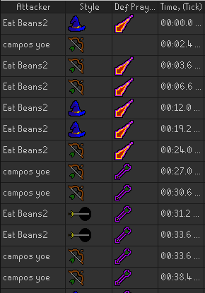
The PvPTracker plugin for the Runelite Client allow us to collect data about combat as we play:
 |
|---|
| Please do not ask about my win/loss ratio |
Each row of the dataset shows the attack style of the attacker and the corresponding defensive prayer of the defender. We have similar tables for many fights.
So it’s easy to extract data that conforms to our idealized representation of combat.
Model Criteria
What do we want our model to do? Well, we want to emphasize simplicity and utility. To keep things simple, let’s focus on predicting only the probability/frequency of attack styles used by opponents.
Then here are some properties of the model that would be nice
- The model predicts the probability of each attack style being used by the opponent
- The model is conditioned on all previous combat data
- The model updates dynamically for each particular opponent based on their actions
This is criteria is relatively simple yet gives us valuable data about our opponent in real time. It also makes use of all of the data available to us.
Such a model also has the potential to be extended. We might instead try to predict conditional attack styles (probability of X attack style if the last attack was Y), or we could design a hierarchical model which uses previous combat data to generate multiple “archetypical profiles” of opponents.
Constructing A Bayesian Model
The model we will construct is an extension of the binomial model described in chapter 1 of Bayesian Data Analysis by Andrew Gelman.
Why Bayesian?
Well, it’s good exercise. But there’s also another reason that I think Bayesian models are well-suited for this problem.
Bayesian models can initialize the prior distribution using data from previous fights, and then we can update the model parameters in real-time using data from the current fight.
In general, I think Bayesian models are an obvious choice when your data comes in the format of “repeated experiments” like this.
Overview of a Bayesian Model
A Bayesian model has a lot of different pieces. If you’re new to this, we’ll quickly describe how a Bayesian model works. Bayesian models revolve around Baye’s theorem:
\[p(\theta\vert y) = \frac{p(y\vert \theta)p(\theta)}{p(y)}\]We will define the components of this equation and then explain the equation itself.
$y$ represents the observations or evidence. We collect samples of $y$, and we want to calculate the probabilities of observing different values of $y$. We should design $y$ to represent not just the data we want (i.e. the next attack style of an opponent) but also the data we intend to condition the model on (i.e. the a quantity of each attack style by an opponent over $n$ attacks).
$p(y\vert \theta)$ is the likelihood or sampling distribution. This is “the model,” in the sense that once we pick some values for $\theta$, this function tells us the probability of any output $y$.
$\theta$ are the model parameters. Our objective is to determine some good values for these using a set of observations of $y$.
$p(\theta)$ is called the prior distribution over model parameters. It represents our beliefs about the model prior to our “training” with collected data. There are many common choices for the prior distribution that we will discuss later.
$p(y)$ is called the marginal likelihood. It’s kind of a wildcard, typically unknown and usually very difficult to approximate.
Finally, $p(\theta\vert y)$ is the posterior. We can calculate this using Baye’s theorem above. It provides us with a means to update our choice of $\theta$ given samples of $y$.
So, here’s our to-do list if we want to build a Bayesian model:
- Craft a sampling distribution $p(y\vert \theta)$ which we think has the capacity to model the situation of interest
- Select a prior distribution $p(\theta)$ which encodes our preexisting beliefs about the model parameters (or, failing that, just pick a mathematically-convenient prior)
- Figure out how to calculate the posterior $p(\theta\vert y)$ using Baye’s theorem
- This will involve approximating or calculating $p(y)$
Once this is all done, the model is ready for action. We can initialize the prior using data from previous fights and then do real-time Bayesian inference during combat.
But I will warn you now; it’s going to be a long journey. Only the most dedicated to Runescape PVP will survive. If you get lost in the sections ahead, you can refer to this section as a roadmap.
Assumptions
Let’s clarify some of the simplifications we are assuming about OSRS combat.
We assume that among $n$ attacks from the opponent, the attack styles are independent and identically distributed (IID). Then the quantities of each attack style constitute a multinomial random variable $y\sim Y$ whose outcomes are $y = [\text{\# Melee},\text{\# Range},\text{\# Mage}]$. The probability of each attack style for a given opponent is unknown.
In reality, this assumption does not hold. For example, each attack by an opponent is probably heavily correlated to their previous attack. However, this model can still provide behavioral insights, and later we will discuss how it can be extended to support these conditional dependencies.
The Likelihood or Sampling Distribution
A simple example: binomial distributions
First we would like to describe the sampling distribution of the opponent’s attacks.
Let’s consider a simpler situation. When a random variable has only two outcomes, we can treat it as a binomial random variable with one parameter, $\theta$, and the sampling distribution is
\[p(y|\theta)={n\choose k}\theta^y (1-\theta)^{n-y} = \frac{n!}{k!(n-k)!}\theta^y (1-\theta)^{n-y}\]This situation is analogous to $n$ (potentially unfair) coinflips where $y$ represents the number of flips resulting in heads. Then $\theta$ represents the probability of getting heads, and $1-\theta$ is the probability of tails. If $\theta=0.5$, it’s a fair coin.
The multinomial distribution
However, in our case we have three outcomes, and thus two parameters, which we denote as
\[\begin{aligned} \theta_{Melee}\text{ or } \theta_{M} \\ \theta_{Range}\text{ or } \theta_{R} \end{aligned}\]where $\theta_{M}+\theta_{R} = 1-\theta_{Magic}$.
Recall that $y$ is a tuple of three integers denoting the quantity of each attack style. For example, if $n=7$, then the outcome $y=[4,2,1]$ means the opponent attacked with Melee 4 times, Range twice, and Mage once. Let $y_i$ denote the $i$th member of $y$.
We are going to write our multinomial sampling distribution using the gamma function instead of factorials. This will make it appear more similar to the other functions (specifically the conjugate prior) later on.
Here is our sampling distribution in all its glory:
\[p(y|\theta_{M}, \theta_{R})=\frac{\Gamma(y_1+y_2+y_3+1)}{\Gamma(y_1+1)\Gamma(y_2 + 1)\Gamma(y_3 + 1)}\theta_{M}^{y_1}\theta_{R}^{y_2} (1-\theta_M - \theta_R)^{y_3}\]The Prior Distribution
There are two obvious choices for the prior distribution $p(\theta_M, \theta_R)$.
The first prior we might consider is the uniform distribution over the standard 2-simplex. This distribution assumes no prior knowledge about the model parameters. In our case, this isn’t really a good fit; we expect to have lots of data from previous experiments to inform our prior.
Another obvious choice is the conjugate distribution of the likelihood. In our case, the likelihood is a categorical distribution, and so the conjugate is a Dirichlet distribution
\[p(\theta_{M}, \theta_{R}) \propto \theta_{M}^{\alpha - 1}\theta_{R}^{\beta - 1} (1-\theta_M - \theta_R)^{\gamma -1}\]Because it is so similar to the likelihood, we can interpret the hyperparameters of this prior distribution. $\alpha-1$ represents the previously-observed quantity of Melee attacks, and similarly for $\beta-1$ and Range, $\gamma-1$ and Magic.
In other words, the conjugate prior makes it very easy to encode previous experiments into the prior distribution. We’re going to use the Dirichlet distribution for our model.
A quick note about normalization: if $\alpha$ is the number of previous melee attacks, etc., then we don’t have a normalized distribution here (which is why I used $\propto$ above instead of $=$). How do we fix this?
Well, the normalizing constant of a Dirichlet distribution is given by $\frac{1}{B(\alpha,\beta,\gamma)}$ where $B$ is the multivariate beta function,
\[\text{B}(\alpha, \beta, \gamma) = \frac{\Gamma(\alpha)\Gamma(\beta)\Gamma(\gamma)}{\Gamma(\alpha + \beta + \gamma)}\]So our complete prior distribution is
\[p(\theta_{M}, \theta_{R}) = \frac{\Gamma(\alpha + \beta + \gamma)}{\Gamma(\alpha)\Gamma(\beta)\Gamma(\gamma)} \theta_{M}^{\alpha - 1}\theta_{R}^{\beta - 1} (1-\theta_M - \theta_R)^{\gamma -1}\]Calculating the Marginal Likelihood
Setup
We’re almost ready to bust out Baye’s theorem and calculate the posterior $p(\theta\vert y)$,
\[p(\theta\vert y) = \frac{p(y\vert \theta)p(\theta)}{p(y)}\]The numerator is known to us. We combine the sampling distribution and prior to give us
\[p(y\vert \theta)p(\theta) = \frac{\Gamma(y_1+y_2+y_3+1)\Gamma(\alpha + \beta + \gamma)\theta_{M}^{y_1}\theta_{R}^{y_2} (1-\theta_M - \theta_R)^{y_3}\theta_{M}^{\alpha - 1}\theta_{R}^{\beta - 1} (1-\theta_M - \theta_R)^{\gamma -1}}{\Gamma(y_1+1)\Gamma(y_2 + 1)\Gamma(y_3 + 1)\Gamma(\alpha)\Gamma(\beta)\Gamma(\gamma)}\]But we can group like terms to reduce this to
\[p(y\vert \theta)p(\theta) = \frac{\Gamma(y_1+y_2+y_3+1)\Gamma(\alpha + \beta + \gamma)\theta_{M}^{y_1 + \alpha - 1}\theta_{R}^{y_2 + \beta - 1} (1-\theta_M - \theta_R)^{y_3 + \gamma - 1}}{\Gamma(y_1+1)\Gamma(y_2 + 1)\Gamma(y_3 + 1)\Gamma(\alpha)\Gamma(\beta)\Gamma(\gamma)}\]But the denominator of Baye’s theorem is trouble. How do we calculate the marginal likelihood, $p(y)$? We could approximate it, but that’s no fun. Can we find an analytical solution? Generally, no, but when using a conjugate prior, the answer is often affirmative.
Recall that we’re calculating a probability distribution over $\theta$. This means that the integral of $p(\theta\vert y)$ with respect to $\theta$ over the domain should be 1,
\[\int p(\theta\vert y)d\theta = \int \frac{p(y\vert \theta)p(\theta)}{p(y)} d\theta = 1\]We can use this constraint to solve for $p(y)$, although it is easier said than done.
Preparing to integrate
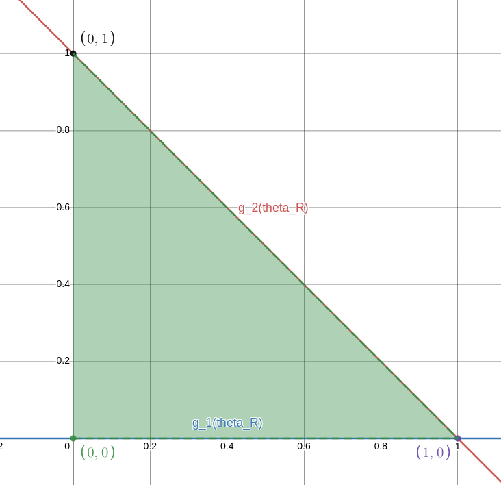
We want to integrate the posterior over all possible values of $\theta_M$ and $\theta_R$. Since our only criteria are $0\leq \theta_M, \theta_R$ and $\theta_M+\theta_R \leq 1$, then the possible values all lie on the triangle contained by $(0,0),(0,1),(1,0)$.
So harkening back to Calculus III, we want to perform a double integration of the posterior from $\theta_R = 0$ to $\theta_R = 1$ on the region contained by $g_1(\theta_R) = 0$ below and $g_2(\theta) = -\theta_R+1$ above.
 |
|---|
| The region over which we are integrating |
So all that’s left is to plop the posterior under a double integral with these bounds. Because $p(y)$ is a constant with respect to $\theta_R$ and $\theta_M$, we can pull it out of the integral immediately: \(\begin{align*} &\int p(\theta\vert y)d\theta =\\ &\frac{1}{p(y)}\int^1_0\int^{-\theta_R+1}_{0} \frac{\Gamma(y_1+y_2+y_3+1)\Gamma(\alpha + \beta + \gamma)\theta_{M}^{y_1 + \alpha - 1}\theta_{R}^{y_2 + \beta - 1} (1-\theta_M - \theta_R)^{y_3 + \gamma - 1}}{\Gamma(y_1+1)\Gamma(y_2 + 1)\Gamma(y_3 + 1)\Gamma(\alpha)\Gamma(\beta)\Gamma(\gamma)} d\theta_M d\theta_R = 1 \end{align*}\)
Tackling the integral
So we need solve the integral, and then we can solve the resulting equation for $p(y)$. Let’s pull out some more constants:
\[\begin{align} \frac{1}{p(y)}\int^1_0\int^{-\theta_R+1}_{0} \frac{\Gamma(y_1+y_2+y_3+1)\Gamma(\alpha + \beta + \gamma)\theta_{M}^{y_1 + \alpha - 1}\theta_{R}^{y_2 + \beta - 1} (1-\theta_M - \theta_R)^{y_3 + \gamma - 1}}{\Gamma(y_1+1)\Gamma(y_2 + 1)\Gamma(y_3 + 1)\Gamma(\alpha)\Gamma(\beta)\Gamma(\gamma)} d\theta_M d\theta_R = \\ \frac{\Gamma(y_1+y_2+y_3+1)\Gamma(\alpha + \beta + \gamma)}{p(y)\Gamma(y_1+1)\Gamma(y_2 + 1)\Gamma(y_3 + 1)\Gamma(\alpha)\Gamma(\beta)\Gamma(\gamma)}\int^1_0\int^{-\theta_R+1}_{0} \theta_{M}^{y_1 + \alpha - 1}\theta_{R}^{y_2 + \beta - 1} (1-\theta_M - \theta_R)^{y_3 + \gamma - 1} d\theta_M d\theta_R \end{align}\]Let’s denote the constant $\frac{\Gamma(y_1+y_2+y_3+1)\Gamma(\alpha + \beta + \gamma)}{\Gamma(y_1+1)\Gamma(y_2 + 1)\Gamma(y_3 + 1)\Gamma(\alpha)\Gamma(\beta)\Gamma(\gamma)}$ as $C$. Now we are dealing with
\[\frac{C}{p(y)}\int^1_0\int^{-\theta_R+1}_{0} \theta_{M}^{y_1 + \alpha - 1}\theta_{R}^{y_2 + \beta - 1} (1-\theta_M - \theta_R)^{y_3 + \gamma - 1} d\theta_M d\theta_R\]The interior integral
Focusing on the interior integral, we can remove the constants to get something like
\[\frac{C\theta_{R}^{y_2 + \beta - 1}}{p(y)}\int^{-\theta_R+1}_{0} \theta_{M}^{y_1 + \alpha - 1}(1-\theta_M - \theta_R)^{y_3 + \gamma - 1} d\theta_M\]This brings to mind an integral of the form
\[\int_0^k t^{a-1}(1-t)^{b-1}dt\]Which is known as the incomplete beta function, a generalization of the beta function. The solution can be expressed in terms of hypergeometric functions.
However, our situation is a slight variant on the incomplete beta function, something like
\(\int_0^k t^{a-1}(c-t)^{b-1}dt = c^{b-1}\int_0^k t^{a-1}(1-\frac{t}{c})^{b-1}dt\) What if we substitute $u = \frac{t}{c}, du=\frac{1}{c}dt$?
\[c^{b-1}\int_0^{k/c} (cu)^{a-1}(1-u)^{b-1}cdu = c^{a+b-1}\int_0^{k/c} u^{a-1}(1-u)^{b-1}du\]Hell yeah, that’s an incomplete beta function! So we can solve the inner integral as an incomplete beta function using substitution. In our case, $c=(1-\theta_R)$. Then
\[\begin{align} \frac{C\theta_{R}^{y_2 + \beta - 1}}{p(y)}\int^{-\theta_R+1}_{0} \theta_{M}^{y_1 + \alpha - 1}(1-\theta_M - \theta_R)^{y_3 + \gamma - 1} d\theta_M = \\ \frac{C\theta_{R}^{y_2 + \beta - 1}(1-\theta_R)^{y_1+y_3+\alpha+\gamma-1}}{p(y)}\int^{1}_{0} \theta_{M}^{y_1 + \alpha - 1}(1-\theta_M)^{y_3 + \gamma - 1} d\theta_M \end{align}\]Surprisingly, the bounds simplified to $0,1$, so this is actually just a boring old beta function, which we can represent as
\[\begin{align} \frac{C\theta_{R}^{y_2 + \beta - 1}(1-\theta_R)^{y_1+y_3+\alpha+\gamma-1}}{p(y)}\int^{1}_{0} \theta_{M}^{y_1 + \alpha - 1}(1-\theta_M)^{y_3 + \gamma - 1} d\theta_M = \\ \frac{C\theta_{R}^{y_2 + \beta - 1}(1-\theta_R)^{y_1+y_3+\alpha+\gamma-1}}{p(y)}B(y_1+\alpha, y_3+\gamma) \end{align}\]The second integral
Alright, so this leaves us with the remaining integral, which turns out to be a beta function as well. How convenient!
\[\begin{align} \frac{C}{p(y)}\int^1_0\int^{-\theta_R+1}_{0} \theta_{M}^{y_1 + \alpha - 1}\theta_{R}^{y_2 + \beta - 1} (1-\theta_M - \theta_R)^{y_3 + \gamma - 1} d\theta_M d\theta_R = \\ \frac{C}{p(y)}B(y_1+\alpha, y_3+\gamma)\int^1_0\theta_{R}^{y_2 + \beta - 1}(1-\theta_R)^{y_1+y_3+\alpha+\gamma-1}d\theta_R = \\ \frac{C}{p(y)}B(y_1+\alpha, y_3+\gamma)B(y_2+\beta, y_1+y_3+\alpha+\gamma) \end{align}\]This appears suspiciously asymmetric at first, but I expanded out the beta functions in terms of gamma functions and discovered that
\[\begin{align} \frac{C}{p(y)}B(y_1+\alpha, y_3+\gamma)B(y_2+\beta, y_1+y_3+\alpha+\gamma) = \\ \frac{C}{p(y)}\frac{\Gamma(y_1+\alpha)\Gamma(y_2+\beta)\Gamma(y_3+\gamma)}{\Gamma(y_1+y_2+y_3+\alpha+\gamma+\beta)} \end{align}\]Which is very pretty and symmetrical, so all is well in the world.
The marginal likelihood
Okay, so finally we are ready to solve the following equation for $p(y)$
\[\begin{align} \int \frac{p(y\vert \theta)p(\theta)}{p(y)} d\theta = \frac{C}{p(y)}\frac{\Gamma(y_1+\alpha)\Gamma(y_2+\beta)\Gamma(y_3+\gamma)}{\Gamma(y_1+y_2+y_3+\alpha+\gamma+\beta)} = 1 \implies\\ p(y) = C\frac{\Gamma(y_1+\alpha)\Gamma(y_2+\beta)\Gamma(y_3+\gamma)}{\Gamma(y_1+y_2+y_3+\alpha+\gamma+\beta)} = \\ \frac{\Gamma(y_1+y_2+y_3+1)\Gamma(\alpha + \beta + \gamma)}{\Gamma(y_1+1)\Gamma(y_2 + 1)\Gamma(y_3 + 1)\Gamma(\alpha)\Gamma(\beta)\Gamma(\gamma)}\frac{\Gamma(y_1+\alpha)\Gamma(y_2+\beta)\Gamma(y_3+\gamma)}{\Gamma(y_1+y_2+y_3+\alpha+\gamma+\beta)} = \\ \frac{\Gamma(y_1+y_2+y_3+1)}{\Gamma(y_1+1)\Gamma(y_2 + 1)\Gamma(y_3 + 1)}\frac{B(y_1+\alpha, y_2+\beta, y_3+\gamma)}{B(\alpha,\beta,\gamma)} \end{align}\]So what? Are we done? How do we know we’re correct?
Validating the marginal likelihood
We can test our formula by comparing to a Monte Carlo approximation. We’ll fix values of $\alpha, \beta, \gamma$ as well as $y_1,y_2,y_3$. Then, we can do a Monte Carlo approximation over the prior to approximate the probability of our $y$ values. It should match the output of this formula.
from scipy.special import gammaln as Gammaln
from scipy.stats import describe
import numpy as np
from numpy.random import default_rng

rng = default_rng()

def marginal_likelihood_prob(y_1, y_2, y_3, alpha, beta, delta):
    '''analytically-derived formula for p(y)'''
    prob = Gammaln(y_1+y_2+y_3+1) - (Gammaln(y_1+1)+Gammaln(y_2+1)+Gammaln(y_3+1))
    prob -= multivar_betaln(alpha, beta, delta)
    prob += multivar_betaln(y_1 + alpha, y_2 + beta, y_3 + delta)
    return np.exp(prob)

def likelihood_prob(y_1, y_2, y_3, theta_m, theta_r):
'''analytically derived formula for p(y|theta)'''
    prob = Gammaln(y_1+y_2+y_3+1) - (Gammaln(y_1+1)+Gammaln(y_2+1)+Gammaln(y_3+1))
    prob += y_1*np.log(theta_m) + y_2*np.log(theta_r) + y_3*np.log(1-theta_m-theta_r)
    return np.exp(prob)

def sample_prior(alpha, beta, delta):
'''generates a random sample from the p(theta) given hyperparameters'''
    return rng.dirichlet([alpha, beta, delta])

def naive_monte_carlo_approx(y_1, y_2, y_3, alpha, beta, delta, n=1000):
'''approximates the marginal likelihood using the prior and monte carlo approximation'''
    probs = []
    for ind in range(0, n):
        theta = sample_prior(alpha, beta, delta)
        probs.append(likelihood_prob(y_1, y_2, y_3, theta[0], theta[1]))
    return probs

if __name__ == '__main__':
y_1, y_2, y_3 = (200, 250, 200)
alpha, beta, delta = (200, 250, 200)

print('Theoretical')
print(marginal_likelihood_prob(y_1, y_2, y_3, alpha, beta, delta))

print('Monte Carlo Simulation')
print(describe(naive_monte_carlo_approx(y_1, y_2, y_3, alpha, beta, delta, n=100000000)))
And the output we get (which took quite a while; you can turn down n for faster results) is
captainofthedishwasher:~$ python3 test_marginal_likelihood.py
Theoretical
0.0006405754905324117
Monte Carlo Simulation
DescribeResult(nobs=100000000, minmax=(1.3299205457019604e-11, 0.0012818163603194933), mean=0.0006406077324059656, variance=1.3696618923819785e-07, skewness=0.0008881199809568082, kurtosis=-1.2002701686108446)
The mean value from the Monte Carlo simulation is a pretty good approximation of the theoretical value. I tested some other values of $y$ and $\theta$ and felt good about the results.
So we’ve finally obtained an analytical formula for $p(y)$. Easy as.
Calculating the posterior
I’m going to be honest with you. The previous section, calculating $p(y)$, was brutal. It took a psychological toll on me. I want to be done. But we are so close. We can do this. Soon we will have a Runescape PVP attack prediction model. I just need to hang in there.
Now that we’ve calculated all of our terms, we’re ready for the whole enchilada: the posterior. Recall once more that we want to calculate $p(\theta\vert y)$ via Baye’s theorem,
\[p(\theta\vert y) = \frac{p(y\vert \theta)p(\theta)}{p(y)}\]And we now know the numerator and denominator:
\[p(y\vert \theta)p(\theta) = \frac{\Gamma(y_1+y_2+y_3+1)\Gamma(\alpha + \beta + \gamma)\theta_{M}^{y_1 + \alpha - 1}\theta_{R}^{y_2 + \beta - 1} (1-\theta_M - \theta_R)^{y_3 + \gamma - 1}}{\Gamma(y_1+1)\Gamma(y_2 + 1)\Gamma(y_3 + 1)\Gamma(\alpha)\Gamma(\beta)\Gamma(\gamma)}\] \[p(y) = \frac{\Gamma(y_1+y_2+y_3+1)}{\Gamma(y_1+1)\Gamma(y_2 + 1)\Gamma(y_3 + 1)}\frac{B(y_1+\alpha, y_2+\beta, y_3+\gamma)}{B(\alpha,\beta,\gamma)}\]Now we need only put them together. I can already see that a lot of terms are going to cancel (thank god)
\[p(\theta\vert y) = \frac{\Gamma(\alpha + \beta + \gamma)B(\alpha,\beta,\gamma)\theta_{M}^{y_1 + \alpha - 1}\theta_{R}^{y_2 + \beta - 1} (1-\theta_M - \theta_R)^{y_3 + \gamma - 1}}{B(y_1+\alpha, y_2+\beta, y_3+\gamma)\Gamma(\alpha)\Gamma(\beta)\Gamma(\gamma)}\]Which, shockingly, simplifies further since we can cancel some multivariate beta functions:
\[p(\theta\vert y) = \frac{1}{B(y_1+\alpha, y_2+\beta, y_3+\gamma)}\theta_{M}^{y_1 + \alpha - 1}\theta_{R}^{y_2 + \beta - 1} (1-\theta_M - \theta_R)^{y_3 + \gamma - 1}\]And there you have it. That’s the posterior. The source of all of our woes and suffering. It’s a boring Dirichlet distribution. What a crazy turn of events! The model is complete. I can’t believe this final step was so easy.
Frankly, I’m not really sure what to do now that we’re here.
Using The Bayesian Model
Oh god, I never thought we’d get this far. I’m really not prepared at all. I’m going to have to put together a dataset and write a program.
Your eyes will simply jump from these sentences to the next as you indulge in the fruits of my labor. Meanwhile, I’m going to have to dig out my laptop, extract all my combat data (if it still exists) to JSON format, figure out how to extract opponent attacks from that, pipe that data into a program, simulate fights, update the posterior, generate some visualizations, structure it all into a narra-
The data
I had a total of 57 fights logged in PvPTracker (I leave my win/loss ratio to the reader’s imagination). The average fight had 24 opponent attacks with a variance of 190, minimum of 3, and maximum of 50. There were a total of 1419 opponent attacks logged.
About 34% of opponent attacks were melee, 39% were ranged, and 27% were magic. This makes sense, as beginners generally consider ranged the “easiest” attack style, while magic is the “hardest”.
I decided we’ll randomly select 10 fights to actually test the model and simulate performing posterior updates during combat. We’ll use the other 47 to determine the prior hyperparameters, $\alpha,\beta,\gamma$.
Initializing the model
$\alpha$ will be the total number of Melee attacks, $\beta$ will the the total of Ranged attacks, and $\gamma$ corresponds to Magic attacks from our 47 prior fights.
Now that the hyperparameters are done, I decided to initialize the model parameters, $\theta_M,\theta_R$ to the expected values of the prior distribution (which is easy to calculate since it’s a Dirichlet distribution), namely
\[\theta_M = \frac{\alpha}{\alpha+\beta+\gamma}, \; \theta_R = \frac{\beta}{\alpha+\beta+\gamma}\]Now our model is fully initialized, and it’s ready to perform inferences and posterior updates!
Posterior updates
Updating $\theta_M,\theta_R$ using the posterior $p(\theta\vert y)$ is actually quite simple. Because the posterior is a Dirichlet distribution, we can update the model parameters to the expected value of the posterior quite easily:
\[\theta_M = \frac{\alpha+y_1}{\alpha+\beta+\gamma+y_1+y_2+y_3}, \; \theta_R = \frac{\beta+y_2}{\alpha+\beta+\gamma+y_1+y_2+y_3}\]Now, I’m trying to stay cool here, but the astute reader has probably observed something quite distressing.
The model is just calculating the average over all attacks. That’s it. There’s no further insights here.
That’s so stupid. What a ripoff. I can’t believe I did all those calculations for a model that an elementary schooler could construct.
Conclusion: This Model Sucks
There’s not much to be said about the data since the model just calculates averages.
The real insight comes from the fact that I wasted so much time deriving this model. How did I do it? Will this happen to me again?
I think that the simplistic outcome should have been predictable from my assumptions. I reduced the problem to a multinomial model, which led to a very simple algorithm. I could probably impose some structure to make the model more interesting, but I’m tired and I want to move on with my life.
Here are some ideas I had for salvaging the model to make it more interesting:
- Make it a hierarchical model where the multinomial parameters for each fight come from another distribution
- Could allow for clustering of opponent behaviors
- Consider correlations between successive attacks instead of independent attacks
- Integrate variables such as health into the model
But these are for another day when I am not so tired. Now, I must rest.