Bernoulli Diffusion Derivations
- What is Bernoulli Diffusion?
- Who is this article for?
- Prependix
- KL divergence of Multivariate Bernoulli Distributions
- $\tilde{\beta}_t$ for Calculating $q\left(\mathbf{x}^{(t)}\vert \mathbf{x}^{(0)} \right)$
- Calculating the Posterior $q\left(\mathbf{x}^{(t-1)}\vert \mathbf{x}^{(t)},\mathbf{x}^{(0)} \right)$
- Entropy of Multivariate Bernoulli Distributions
What is Bernoulli Diffusion?
Short answer: a Github repo that I made.
Long answer:
Diffusion originated from the classic publication Deep Unsupervised Learning using Nonequilibrium Thermodynamics by Sohl-Dickstein et al.
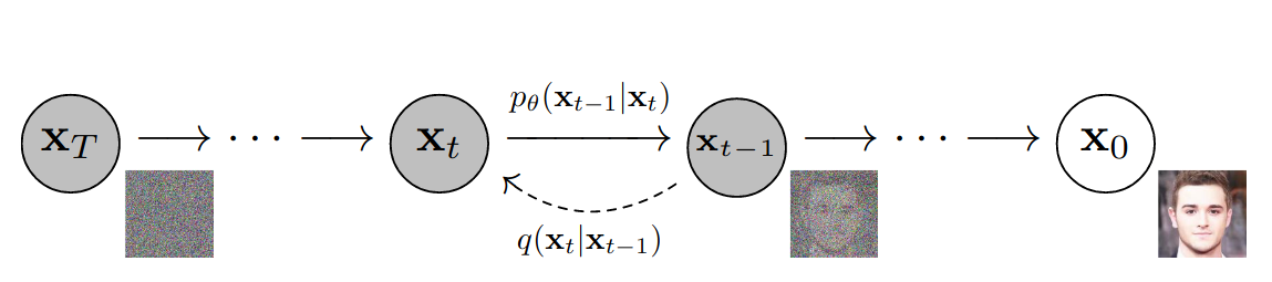
In the original paper–as well as most practical applications of diffusion (see stable-diffusion)–a Gaussian Markov diffusion kernel is used. This means the algorithm iteratively applies Gaussian noise to samples from the target distribution and then learns to reverse the noising process.
 |
|---|
| An illustration of Gaussian diffusion stolen from this paper. You’re legally required to put this in any technical article about diffusion. |
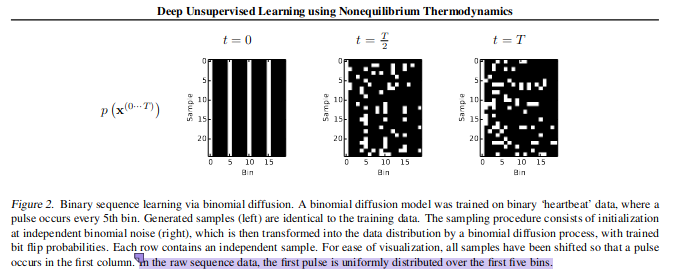
However, the original paper offhandedly mentions that you can also implement diffusion for binary-valued data using a Bernoulli distribution as your Markov diffusion kernel.
 |
|---|
| A segment of the original diffusion paper which mentions using Bernoulli diffusion to learn “heartbeat data”. |
The authors of the paper published the code for the Gaussian diffusion, but for some reason chose not to publish the Bernoulli diffusion model. I have yet to find an implementation of Bernoulli diffusion anywhere on the internet.
So I decided to implement it myself. It was very hard. I calculated a lot of things and learned a lot of fancy new words.
Here I will be detailing some of the more interesting derivations that I haven’t seen documented anywhere else.
Who is this article for?
Me. I need to dump this all somewhere so that I can finally forget it. However, it might help if you are trying to understand the code in the Bernoulli Diffusion repo. One day in the distant future, these notes might even help college students cheat on their homework.
Prependix
Most of these calculations have to do with the terms involved in this the loss approximation (equation 14 in the paper):
\[K = -\sum_{t=2}^T\int d\mathbf{x}^{(0)} d\mathbf{x}^{(t)} q\left(\mathbf{x}^{(0)}, \mathbf{x}^{(t)} \right)\cdot \\ D_{KL}\left(q\left(\mathbf{x}^{(t-1)}\vert \mathbf{x}^{(t)},\mathbf{x}^{(0)} \right) \vert \vert p\left(\mathbf{x}^{(t-1)}\vert \mathbf{x}^{(t)}\right)\right) \\ + H_q(\mathbf{X}^{(T)}\vert \mathbf{X}^{(0)}) - H_q(\mathbf{X}^{(1)}\vert \mathbf{X}^{(0)}) - H_p(\mathbf{X}^{(T)})\]So I figured I’d prepend it here for reference later.
KL divergence of Multivariate Bernoulli Distributions
In order to calculate $K$, we will need to calculate
\[D_{KL}\left(q\left(\mathbf{x}^{(t-1)}\vert \mathbf{x}^{(t)},\mathbf{x}^{(0)} \right) \vert \vert p\left(\mathbf{x}^{(t-1)}\vert \mathbf{x}^{(t)}\right)\right)\]Where $q\left(\mathbf{x}^{(t-1)}\vert \mathbf{x}^{(t)},\mathbf{x}^{(0)} \right)$ and $p\left(\mathbf{x}^{(t-1)}\vert \mathbf{x}^{(t)}\right)$ are both essentially a bunch of Bernoulli distributions.
I actually found the answer here, so I’m not going to elaborate on this one.
$\tilde{\beta}_t$ for Calculating $q\left(\mathbf{x}^{(t)}\vert \mathbf{x}^{(0)} \right)$
Okay, so in this paper the authors casually remark that the forward process in Gaussian diffusion has a really nice computational property. Specifically, if
\[q\left(\mathbf{x}^{(t)}\vert \mathbf{x}^{(t-1)} \right) =\mathcal{N}\left(\mathbf{x}^{(t)};\sqrt{1-\beta_t}\mathbf{x}^{(t-1)}, \beta_t\mathbf{I}\right)\]then you can define $\alpha_t := 1-\beta_t$ and $\bar{\alpha_t} := \prod_{s=1}^{t} \alpha_{s}$, and it follows that
\[q\left(\mathbf{x}^{(t)}\vert \mathbf{x}^{(0)} \right) =\mathcal{N}\left(\mathbf{x}^{(t)};\sqrt{\bar{\alpha}_t}\mathbf{x}^{(0)}, (1-\bar{\alpha}_t)\mathbf{I}\right)\]So, in other words, you don’t have to iterate the forward noising process $t$ times to get a sample $\mathbf{x}^{(t)}$. You can just sample it directly.
I figured something similar held for the Bernoulli case. However, the authors didn’t actually demonstrate how this relationship is derived. I’ll leave the Gaussian case as an exercise and show the Bernoulli case instead.
We can focus on an individual digit $\mathbf{x}^{(t)}_i$. The way I derived this was by denoting
\[\mathbf{x}^{(t)}_i = \mathbf{x}^{(t-1)}_i(1-\epsilon_t) + (1-\mathbf{x}^{(t-1)}_i)\epsilon_t = \mathbf{x}^{(t-1)}_i + \epsilon_t - 2\epsilon_t \mathbf{x}^{(t-1)}_i\]Where $\epsilon_t = \mathcal{B}(0.5\beta_t)$ is a Bernoulli random variable. This is just another way of representing the typical noising process as a probability of flipping bits.
I used this recursively to represent $\mathbf{x}^{(t+1)}_i$ in terms of $\mathbf{x}^{(t-1)}_i$ and then simplified to find that:
\[\mathbf{x}^{(t+1)}_i = \mathbf{x}^{(t-1)}_i + \epsilon_t + \epsilon_{t+1} - \epsilon_t \epsilon_{t+1} - 2(\epsilon_t + \epsilon_{t+1} - \epsilon_t \epsilon_{t+1})\mathbf{x}^{(t-1)}_i\]denoting $\tilde{\epsilon}_ {t+1} := \epsilon_t + \epsilon_{t+1} - \epsilon_t \epsilon_{t+1}$, we see that
\[\mathbf{x}^{(t+1)}_i = \mathbf{x}^{(t-1)}_i + \tilde{\epsilon}_{t+1} - 2\tilde{\epsilon}_{t+1}\mathbf{x}^{(t-1)}_i\]Which is the same relationship as the original case! If we wanted to skip even further, say from $\mathbf{x}^{(t-1)}$ to $\mathbf{x}^{(t+2)}$, then we would derive that
\[\mathbf{x}^{(t+2)}_i = \mathbf{x}^{(t-1)}_i + \tilde{\epsilon}_{t+1} + \epsilon_{t+2} - {\epsilon}_{t+1}\epsilon_{t+2} - 2(\tilde{\epsilon}_{t+1} + \epsilon_{t+2} - {\epsilon}_{t+1}\epsilon_{t+2})\mathbf{x}^{(t-1)}_i\]So generally we have that
\[\tilde{\epsilon}_ {t+1} = \tilde{\epsilon}_{t} + \epsilon_{t+1} - \tilde{\epsilon}_{t}\epsilon_{t+1}\]Then the corresponding Bernoulli distribution is
\[\mathcal{B}(0.5(\tilde{\beta}_{t} + \beta_{t+1} - \beta_{t+1}\tilde{\beta}_{t})) := \mathcal{B}(0.5\tilde{\beta}_{t+1})\]And we have a recursive relationship for our desired values,
\[\tilde{\beta}_{t+1} = \tilde{\beta}_{t} + \beta_{t+1} - \beta_{t+1}\tilde{\beta}_{t}\]Then
\[q\left(\mathbf{x}^{(t)}\vert \mathbf{x}^{(0)} \right) =\mathcal{B}\left(\mathbf{x}^{(0)}(1-\tilde{\beta}_{t}) + 0.5\tilde{\beta}_{t}\right)\]Badda bing, badda boom.
Calculating the Posterior $q\left(\mathbf{x}^{(t-1)}\vert \mathbf{x}^{(t)},\mathbf{x}^{(0)} \right)$
Another obstacle while computing the loss $K$ is the posterior,
\[q\left(\mathbf{x}^{(t-1)}\vert \mathbf{x}^{(t)},\mathbf{x}^{(0)} \right)\]Where $\mathbf{x}$ and $\mathbf{x}^{(t)}$ are given. The first time I saw this, I had no idea how to even interpret it, and the authors never even mention it beyond “oh, yeah, that’s the posterior.”
But contextually, it seems like it should be analytically computable, and in fact you can find a computation of the posterior in the source code of the Gaussian diffusion repo.
I eventually realized that the authors don’t mention it because it’s trivial to a keen Bayesian statistican. Essentially, you can think of this as a tiny Bayesian model within the larger system. The inspiration came to me while reading Bayesian Data Analysis, by Andrew Gelman, particularly section 2.5. This is coincidentally almost exactly the solution for the Gaussian posterior.
Usually with a Bayesian system, you construct a sampling model $p(y\vert \theta)$ dependent on the parameters $\theta$. Then you establish a prior distribution on the parameters $p(\theta)$.
When you finally collect data $y$ and want to determine the proper parameters $\theta$, you’ll need to calculate the posterior distribution (or something proportional to it):
\[p(\theta \vert y) = \frac{p(y\vert\theta)p(\theta)}{p(y)}\]we can translate this into our current case as follows:
\[y = \mathbf{x}^{(t)} \\ \theta = \mathbf{x}^{(t-1)} \\ p(\theta) = q\left(\mathbf{x}^{(t-1)}\vert \mathbf{x}^{(0)} \right) = \mathcal{B}\left(\mathbf{x}^{(0)}(1-\tilde{\beta}_{t-1}) + 0.5\tilde{\beta}_{t-1}\right) \\ p(y\vert \theta) = q\left(\mathbf{x}^{(t)}\vert \mathbf{x}^{(t-1)},\mathbf{x}^{(0)} \right) = \mathcal{B}\left(\mathbf{x}^{(t-1)}(1-\beta_{t}) + 0.5\beta_{t}\right) \\ p(\theta\vert y) = q\left(\mathbf{x}^{(t-1)}\vert \mathbf{x}^{(t)},\mathbf{x}^{(0)} \right) \\ p(y) = q\left(\mathbf{x}^{(t)}\vert \mathbf{x}^{(0)} \right)\]Now the given variables, $\mathbf{x}^{(t)}$ and $\mathbf{x}^{(0)}$, determine a prior distribution and a set of observations, so we can get to work calculating the posterior
\[p(\theta \vert y) = \frac{q\left(\mathbf{x}^{(t)}\vert \mathbf{x}^{(t-1)},\mathbf{x}^{(0)} \right)q\left(\mathbf{x}^{(t-1)}\vert \mathbf{x}^{(0)} \right)}{q\left(\mathbf{x}^{(t)}\vert \mathbf{x}^{(0)} \right)}\]Since we parameterize the Bernoulli distributions using the probability of observing 1, want to calculate $p(\theta =1\vert y)$ and thus we set $\mathbf{x}^{(t-1)} = 1$.
I also ended up calculating the cases for $\mathbf{x}^{(t)} = 1$ and $\mathbf{x}^{(t)} = 0$ separately because it seemed easier. Then I combined them into a single equation:
posterior = x_0*(1-self.beta_tilde_t[t-1]) + 0.5*self.beta_tilde_t[t-1]
posterior *= x_t * (1-0.5*beta_t) + (1 - x_t) * (0.5*beta_t)
normalizing_constant = x_t * self.q_conditional_prob_wrt_x_0(x_0, t) + (1-x_t) * (1-self.q_conditional_prob_wrt_x_0(x_0, t))
posterior = posterior / normalizing_constant
Honestly, I’m still not totally sure if this needs to be normalized or something. I should probably put that on my long list of to-dos. EDIT (11/3/2022): The former documentation has been updated and now describes how to calculate a normalized posterior. I did, indeed, need to normalize the posterior. I spent an entire month trying to figure out why my diffusion implementation was apparently experiencing mode collapse. It was because the posterior needed to be normalized.
Often, the normalization factor is intractable, so it is purposefully ommitted in many discussions of posterior calculation. It is very easy to calculate in this case, and I should have checked before assuming we did not need it.
Do not be like me. Check whether the normalization factor is tractable.
Entropy of Multivariate Bernoulli Distributions
This one was a doozy. While calculating that darn $K$ value, we find ourselves in need of the following entropies:
\[H_q(\mathbf{X}^{(T)}\vert \mathbf{X}^{(0)}) - H_q(\mathbf{X}^{(1)}\vert \mathbf{X}^{(0)}) - H_p(\mathbf{X}^{(T)})\]These are entropies of multivariate Bernoulli distributions. So, first thing’s first, the definition of the entropy of a discrete distribution $p(x)$ over $\mathcal{X}$ is
\[H(p(x)) = -\sum_{x\in\mathcal{X}}p(x)\log p(x)\]Now, for a single Bernoulli distribution with probability $0\leq c \leq 1$, it works out that
\[H(\mathcal{B}(c)) = -(c\log c + (1-c) \log (1-c))\]But life is not so simple when you get to the multivariate case. If we have $n$ Bernoulli distributions, each with probability $p_i$, then the probability of an outcome $x\in\{0,1\}^n$ is given by
\[p(x) = \prod_{i=1}^n x_i p_i + (1-x_i)(1-p_i)\]and there are $2^n$ values of $x$ in our entropy summation… If we are learning sequences of length 20, each loss calculation would involve summing $2^{20}=1048576$ products. That is not efficient.
However! There are additional constraints at play which give us hope.
Let’s consider $H_q(\mathbf{X}^{(T)}\vert \mathbf{X}^{(0)})$. Recall that
\[q\left(\mathbf{x}^{(T)}\vert \mathbf{x}^{(0)} \right) = \mathcal{B}\left(\mathbf{x}^{(0)}(1-\tilde{\beta}_{T}) + 0.5\tilde{\beta}_{T}\right)\]Consequently, each Bernoulli distribution can only have one of two probabilities:
\[p_i = \begin{cases} 1-0.5\tilde{\beta}_T, & \text{if} & \mathbf{x}^{(0)}_i = 1 \\ 0.5\tilde{\beta}_T, & \text{if} & \mathbf{x}^{(0)}_i = 0 \end{cases}\]It follows almost immediately that $\mathbf{x}^{(T)}_i = \mathbf{x}^{(0)}_i$, then the probability must be $1-0.5\tilde{\beta}_T$, and otherwise the probability of $\mathbf{x}^{(T)}_i$ is $0.5\tilde{\beta}_T$.
In other words, the probability of any outcome $\mathbf{x}^{(T)}$ is totally determined by the number of digits it has in common with $\mathbf{x}^{(0)}$. If they agree in $k$ digits and disagree for the other $k-n$, then the probability of $\mathbf{x}^{(T)}$ is
\[(1-0.5\tilde{\beta}_T)^k (0.5\tilde{\beta}_T)^{n-k}\]So how many samples will have each probability? a bit of thought will convince you that there is $n$ choose $k$ ways to agree in $k$ digits.
Now, how does this all tie back into entropy? Well, all three entropies are similar, but wrapping up the case of $H_q(\mathbf{X}^{(T)}\vert \mathbf{X}^{(0)})$, we can calculate that
\[H(p(x)) = -\sum_{x\in\mathcal{X}}p(x)\log p(x) \\ =-\sum_{k=0}^n {n\choose k}(1-0.5\tilde{\beta}_T)^k (0.5\tilde{\beta}_T)^{n-k}\log \left((1-0.5\tilde{\beta}_T)^k (0.5\tilde{\beta}_T)^{n-k}\right)\]Easy as.