The Inscribed Rectangle Proof, Visually
- Introduction
- Turning Points on a Loop Into Rectangles
- The Existence Question
- Intermission: Gathering Information With Topology
- Twisting $L$ and $L_{\phi}$ Into Mobius Strips
- Smoothing Out the Trivial Intersection
- I’m Not Trained In Symplectic Geometry
- An Abrupt End
Introduction
This post is about an amazing modern proof published by Joshua Evan Greene and Andrew Lobb. Their statement is simple, as far as mathematical papers go:
Let’s rephrase this in (approximately equivalent) human terms: Draw a smooth loop on a piece of paper. Now, pick a rectangle of some length:height proportion. A simple example might be 1:1, which is a square. 2:1 would be a little more rectangle-y. The claim is that you can find 4 points on your loop which make a rectangle of that proportion. This sounds a little zany, so let’s look at an example.
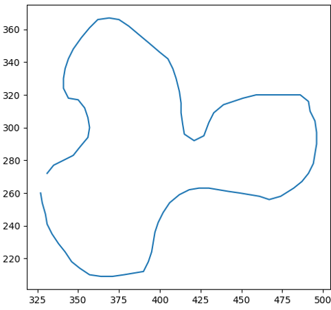
First, here’s your curve:
Now, let’s start simple. Can we find a square? We sure can!
Keep in mind that the method used to find our shapes is algorithmic, and it’s not perfect, but the proof that these shapes exist is perfect. Let’s find a more rectangular rectangle. From now on, we will describe the proportions of a rectangle by the angle between its diagonals. For example, a square would be 90 degrees or $\pi /2$ radians. We will refer to this angle as $\phi$ (pronounced “fee,” if you were wondering). Let’s try a rectangle with $\phi = \pi /4$
So far, so good! But we won’t much much further by picking more rectangles. If we want to see why this is true, we need to start digging into the actual proof. We’ll ease into it by talking about what a rectangle really is in the eyes of these mathematicians.
Turning Points on a Loop Into Rectangles
A Particular Method of Searching
I find one convenient way to begin down this long road is by asking an intuitive question: how would you search for an inscribed rectangle on some loop? Your first instinct might be along the lines of
- Pick four points on the loop
- Check if they form a rectangle
- Check if the diagonal’s angle, $\phi$, is correct
- Repeat
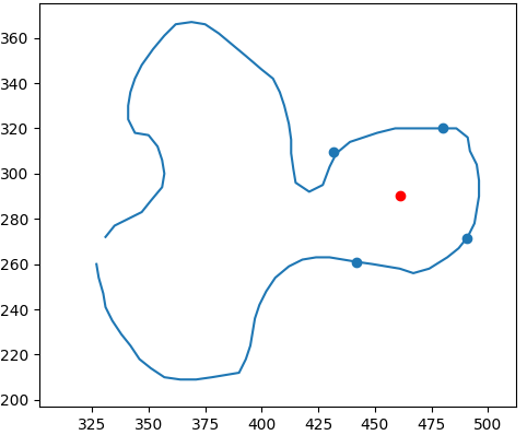
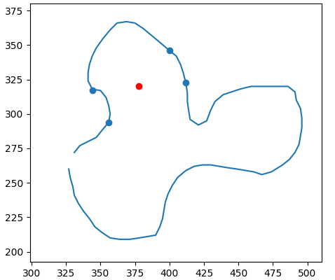
This is hypothetically a sufficient method to go about finding your rectangle. It might take a very long while, but that doesn’t bother mathematicians. However, it is not very refined. say on step one you’ve picked two points on your loop and have two more to choose. You can immediately tell that most other points would not be a good choice! Once you’ve picked two points, there’s actually only two pairs of points on your piece of paper that would give you a rectangle of the desired proportions, and all you need to know is whether those points are on the curve too. Here’s an example where we’re searching for a rectangle with angle $\phi=\pi /4$. We’ve already picked two points, and we can see the only possible rectangles with the right proportions.
Those two points are, consequently, not the ones we’re looking for. This method narrows our search a little bit, which is nice. However, the reason this method is important is because it’s more distilled. When we were picking four points at a time, there was a lot of excess information that wasn’t relevant, since two points already told us what we wanted to know. We’re doing some housekeeping on the information relevant to our problem before we start building theory.
Calculating the Two Rectangles for a Pair of Points
I’m sure you’re all asking, “but given $\phi$ and a pair of points, how can we mathematically determine these two rectangles?” Well, I’ll tell you. In the paper, the authors use complex numbers to make the arithmetic more convenient. We’ll do that too, but you could also answer this with boring old geometry in cartesian coordinates if you desired. There are two rectangles, so we’ll describe two processes and give them each a name. This is straight out of the original paper, so get excited: you’re doing math!
The first thing we do is convert coordinates into complex numbers, $(a,b)\rightarrow a+bi$. Pretty easy, right? so our pair of points might go
Notice we renamed the two points $z$ and $w$ now that they’re just complex numbers.
Rectangle One
First we are going to calculate two intermediate values. These intermediate values will then give us all four points on the rectangle. For the first rectangle, these values are given by
So now we’ve got two new complex numbers, which we named $p$ and $q$. If you want your rectangle from these two points, here is how you get them. The first two rectangle points are given by $p+q$ and $p-q$. But that’s boring, since these are just the two points we started with (check it yourself). To get the other two points, we’re going to rotate $q$ and then do the same adding and subtracting.
Remember that a complex number like $p$ can also be described by a distance and an angle, $r$ and $\theta$. We switch to that notation here because it’s a lot easier to write a rotation function. When we switch notations, we’ll write $q$ like $(r_q, \theta_q)$. Try to remember that those are exactly the same things.
So, we rotate $q$ by $-\phi$ (negative simply to keep consistent with the paper; don’t panic). We can express this as $(p,q)\rightarrow (p, r_q, \theta_q-\phi)=(p,q’)$. Then, finally, the last two points of our rectangle are $p+q’$ and $p-q’$.
I won’t dwell on why this works for too long. You should be able to calculate why the first two rectangle points work. As for the second two points, the idea is that we’re reorienting to get the points on the other diagonal, which is why the angle between diagonals, $\phi$, is involved. I encourage you to explore further on your own.
Rectangle Two
One more rectangle to go! This process is very similar to the previous, but we add one more step. Our last construction implicitly assumed which diagonal (a rectangle has two) our original pair of points were on. We’re now going to assume they’re on the other diagonal. To do this, we start with the function $l:(z, w)=(p,q)$ as before. Now we’re adding a new step: another rotation. Define a function that just rotates the $p$ in $(q,p)$ forward by an angle of $\phi$:
Then we rotate $q$ again, but this time by $-\phi$, just like our first rectangle. Then, finally, the last two points of our rectangle are $p+q’$ and $p-q’$. The astute reader might be thinking, “hey, didn’t we just rotate $q$ by $\phi$ and then by $-\phi$? Isn’t that redundant?” It sure is, but I wanted to stay true to the notation of the actual paper, which leads us into this awkward discussion. What matters is that you notice $q$ is rotated by a different amount (a difference of $\phi$) in Rectangle One vs. Rectangle Two.
Summary
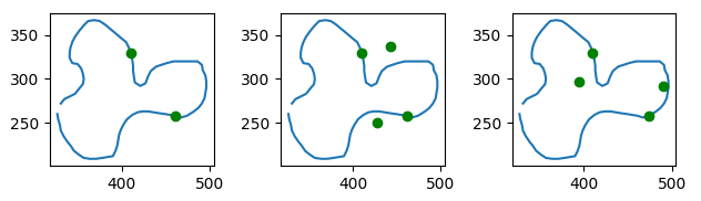
So we’ve started laying the groundwork for talking about rectangles on loops. We found out that, once you pick a diagonal angle $\phi$, every pair of points $z$ and $w$ can be on two possible rectangles. We calculate the vertices of these two rectangles using two intermediate pairs of points: $l(z,w)$ and $R_{\phi}(l(z,w))$. Each intermediate pair, call them $p,q$, is converted to a rectangle by calculating $p \pm q$ and $p \pm (r_q, \theta_q-\phi)$. Here’s an overview animation of the process we just described for a bunch of different pairs of points:
The top row shows our selection of two points. In columns one and two, we see the construction of rectangles one and two, respectively. In particular, we build the two $p$ and $q$ points that we will be adding and subtracting to get rectangle vertices. Finally, we see the corresponding rectangle.
As an important sidenote (which we’ll return to later): keep in mind what happens if you plug a pair of the same point, $(z,z)$ into $l(z,z)$ and $R_{\phi}(l(z,z))$. Specifically, you build a “rectangle” with zero width and zero height. Your intermediate point is always $(z,0)$ for both Rectangle processes. This edge case will need to be addressed later, but you can forget it for most of the next section.
We’re cooking now!
The Existence Question
Beginning With Pairs on the Loop
We’ve been talking about how one might search for a rectangle with the desire proportions, but we haven’t talked about whether such a rectangle actually exists. This is a pretty big gap to leap. The success of the proof is due partly to the fact that they rephrased the existence question in a way that hinted how one might investigate further.
With our understanding from the previous section, we’re ready to start asking the big questions as well. Keep in mind our two processes for creating a rectangle from points. We call them Rectangle One and Rectangle Two processes for now.
Let’s start building the existence proof. We first make some observations about the Rectangle processes. Suppose during our search that we picked a pair of points and found that they did, in fact, yield the desired rectangle on our loop. By the Rectangle processes above, our two points will be one of the diagonals.
Here is the interesting part: if we had to use the Rectangle One process to get the right result from our pair, then we could also use the Rectangle Two process on the other diagonal pair to get the same rectangle, and vice versa. So we could have found either diagonal pair to solve our problem. Going further, the two diagonal pairs of the rectangle must use opposite Rectangle processes (check this, if you please). However, you get the same rectangle and the same intermediate points (since these uniquely determine the rectangle).
This may sound really elaborate, but we’re making this argument because we can now phrase the existence problem within a very neat mathematical framework. The punchline is this:
To rephrase this one more time, a rectangle exists on the loop if there are two pairs such that you can apply the Rectangle One process to one pair and the Rectangle Two process to the other and get the same intermediate values. Here’s a picture to illustrate this concept. The top row is two pairs of points which form the diagonals of the same rectangle. The middle row is the intermediate values, except the first pair used the Rectangle One process while the other pair used the Rectangle Two process. Finally, we see they generate the same rectangles by the opposite processes.
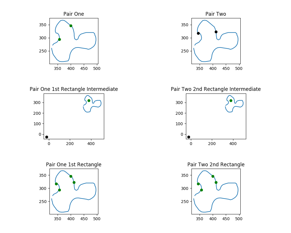
So, here’s the punchline: if we want to show that a rectangle of the desired proportion exists, all we need to show is that there’s some $(a,b)$ and $(c,d)$ on the curve such that $l(a,b) = R_{\phi}(l(z,w))$. To tackle this problem, we’re going to leave behind points on the curve and start talking about the spaces of possible intermediate points, $l(z_1,w_1)$ and $R_{\phi}(l(z_2,w_2))$. Another way to word our problem is that we’re trying to show that their intersection is non-empty, meaning they share a point somewhere.
Rephrasing With Intermediate Values
We now know that finding a rectangle with diagonal angle $\phi$ is equivalent to finding a shared pair of points between $l(z_1,w_1)$ and $R_{\phi}(l(z_2,w_2))$. Thus far, we’ve taken points from our loop one pair at a time and plugged them into these formulas. Since we’re looking for the intersection of these two spaces, we need to think bigger.
We’re going to take all the pairs of points off the loops, plug them into $l(z_1,w_1)$, and call resulting blob of pair of intermediate values $L$. We can make this more rigorous: if $\lambda$ is all the points on our curve, then $\lambda \times \lambda$ is the set of all pairs of points, and $L=l(\lambda \times \lambda)$. We also define something similar for the other equation, $L_{\phi} = R_{\phi}(l(\lambda \times \lambda))$.
Thus, we have two blobs, which are each composed of pairs of complex numbers received by plugging into our two Rectangle processes.
\[L=l(\lambda \times \lambda) \quad L_{\phi} = R_{\phi}(l(\lambda \times \lambda))\]This may seem a little abstract, so the following visualizations show how these blobs relate to our original curve. We trace a path along pairs of points in the original curve, and we observe the resulting points in $L$ and $L_{\phi}$. How we represent our intermediate points is a little different from how we plotted our original pairs of points. We give each of the intermediate points its own graph, because we want to leave room to see all the possible pairs at once.
The colored blob was drawn by the tracing process illustrated in the images. It’s very important to observe the color gradient. Only pairs which were drawn simultaneously–and thus which have the same color–are valid pairs. You cannot pick any arbitrary point from each blob and mash them together.
So, in summary, our spaces $L$ and $L_{\phi}$, the collections of possible intermediate values, are each represented by two colorful blobs. Each blob is all possible values of one point in the pair of points. For $L$ or $L_{\phi}$, you can match intermediate pairs between the two blobs by finding points with identical colors.
You should keep in mind that the plots here are not perfect: you can see that the path overlaps itself, and thus previous colors in a spot get wiped out by later colors. As a result, you can’t see all of the valid pairs of points. This method is imperfect because the pairs of complex-valued points actually sit in 4-dimensional space. I’m strapping together two 2-dimensional planes and calling it close enough. This model is sufficient for expressing many of the ideas to come.
Now, how do we rephrase our original goal to fit these pretty pictures? We’re trying to find pairs of points on L (remember they must match in color) which are in the same positions as a pair of points on $L_{\phi}$ (which must have their own matching color). This is the intersection of $L$ and $L_{\phi}$. We can leave behind our original points and start thinking about $L$ and $L_{\phi}$ alone.
This is a good point to remind you of the interesting exception mentioned at the end of the previous section. The intersection of $L$ and $L_{\phi}$ will contain any solution rectangles, but it also contains any pair $(z,0)$. This maps to a rectangle of zero width and zero height! And these have any proportion to each other you’d like.
Plugging in $(z,z)$ will give you the point $(z,0)$ for both $L$ and $L_{\phi}$. Later on, we will “remove” these points before we finish our search for the actual solution. In fact, we’re actually going to leverage the fact that we know $L$ and $L_{\phi}$ have intersect along these points, $\lambda \times {0}$. We’ll use this set of intersections to stitch these two data sets together. Then we’ll do some topology fun on the conjoined blobs!
Intermission: Gathering Information With Topology
So we’ve got two collections of pairs of points, $L$ and $L_{\phi}$, and the inscribed rectangle existence question has been made equivalent to the question of whether $L$ and $L_{\phi}$ share any pairs. Why have we done all of this awkward rephrasing? Well, believe it or not, mathematicians have a lot of tools for handling questions like this.
In this section, we’re going to start invoking some tools of topology to describe our $L$ and $L_{\phi}$ spaces. Although the concepts are somewhat abstract, our visual guides will help keep us grounded. We’re going to establish that most of the things we’ve been looking at are some kind of torus. We’re going to remove redundancies by using a function to twist $L$ and $L_{\phi}$ into Mobius strips.
Later on, we will combine the sets $L$ and $L_{\phi}$ together and erase the trivial intersection we found, $\lambda \times {0}$. Then we’re going to twist the $L$ and $L_{\phi}$ parts of the conjoined blob each into a mobius strip by mapping them with a function.
At this point we are very near the heart of the proof. The general idea is that when $L$ and $L_{\phi}$ are each twisted into mobius strips, and since we have combined them and removed the trivial intersection along $\lambda \times {0}$, the resulting object is a Klein bottle (Here is a brief summary of how a Klein bottle is made from two mobius strips). But since we’re in 4-dimensional space ($\mathbb{C}^2$), the Klein bottle has to intersect itself. However, this means that $L$ and $L_{\phi}$ have to intersect each other, thus solving the existence problem!
The Shape Of Our Data
So we’re going to start by describing the shape of our sets of points, $L$ and $L_{\phi}$. I’d like the reader to keep something in mind as we go on. All of the animations you’ve seen of $L$ and $L_{\phi}$ have appeared to be a line tracing out a path. However, this is due to the fact that we’re using computers who can’t sample all of the (infinite) positions on our curve. If we could do that, we’d end up with smooth, colored surfaces rather than the dense weavings of a single line. That being said, what is the shape of these surfaces?
Let’s start simpler by considering all the pairs of points on our original curve. Remember we call the set of all of these pairs $\lambda\times\lambda$. This shape is somewhat easier to imagine. Suppose you’ve picked some pair of points. You can “walk” the first point back and forth on the curve, or you can “walk” the second point back and forth. If either point “walks” in a full loop, you end up exactly back where you started. In this sense, there are two distinguished kinds of loop you can walk in: one with the first point, and one with the second point.
What kind of shape has two distinguished loops to walk around? A torus! A torus is what a mathematician calls the surface of a doughnut. On a torus, you can either walk a loop around the hole in the center, or you can walk a loop through the center. These two kinds of loops are distinct in the sense that you can’t smoothly vary one into the other. The following is a picture pulled from Wikipedia which shows these two kinds of loop. Keep in mind the loops have to stay on the surface of the doughnut, and try to imagine smoothly deforming one into the other. You should find it impossible!
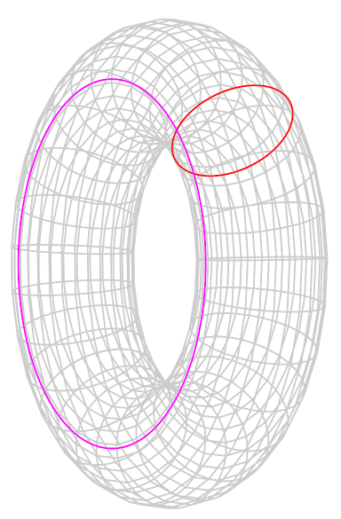
The visually (or topologically) inclined might be able to see why $\lambda\times\lambda$ is a torus. It’s the product of two loops, i.e. “a circle of circles.” Otherwise, I hope you can believe that $\lambda\times\lambda$ is some kind of lumpy, weird torus because it has two distinct kinds of loops you can trace out.
At the risk of oversimplifying, it follows pretty quickly that $L$ and $L_{\phi}$ are tori as well. Remember that these are given by $L=l(\lambda\times\lambda)$ and $L_{\phi}=R_{\phi}(l(\lambda\times\lambda))$. Our functions are a special kind of function: $l$ and $R_{\phi}$ don’t destroy any of the shape properties of our data. We call functions like this “homeomorphisms.” We can say in our case that all of these sets are homeomorphic to each other and to a torus. So loops of one kind map to loops of the same kind through the functions, and we end up with the same two distinct classes of loop.
Here’s a plot tracing out an example of the two kinds of loop on our new, weirder tori. You can see I move each of the two points on the original curve in a full loop, and our homeomorphism means we will see two distinct loops on our new sets, in this example, $L$.
So now we know we’re looking at a bunch of tori. Why do we want to know this? We’re going to do some twisting of these tori (specifically $L$ and $L_{\phi}$) in order to turn them into Mobius strips. Once we’ve done that, the last big hurdle will be combining $L$ and $L_{\phi}$ together and erasing thetrivial intersection along $\lambda \times {0}$. Then when we twist $L$ and $L_{\phi}$ into mobius strips, the combination will be a klein bottle, and the self-intersection of the Klein bottle will prove the existence of our desired rectangle!
Twisting $L$ and $L_{\phi}$ Into Mobius Strips
Who Invited Mobius, Anyways?
So we’ve got one more function we’ll be using to “change our perspective.” That function is
So what’s this all about? Why do we need to do more mapping? Well, recall that for each pair of intermediate points (i.e. pair in $L$ or $L_{\phi}$, there are two pairs of corresponding points on the curve (i.e. the two diagonals of the respective rectangle). However, there has been an oversight in our $L$ and $L_{\phi}$ mappings! I have hidden a problem from you. Specifically, suppose you have some pair $(z,w)$ on the loop. Then logically, $l(z,w)$ and $l(w,z)$ ought to give you the same intermediate points, since $(z,w)$ and $(w,z)$ obviously share the same rectangles. But $l(z,w)$ and $l(w,z)$ aren’t equal!
It’s easy to see that $l(z,w)$ and $l(w,z)$ are different from the definition of $l$. The first term is the same in either case. However, the second term will flip from positive to negative or vice versa along both axes. So why are we talking about this? Even if they produce different intermediate points, you get the same rectangles either way, right? Well, we’re talking about it because this means our sets of intermediate values, $L$ and $L_{\phi}$ have excess information. If we don’t care whether the pair is $(z,w)$ or $(w,z)$, then our data set shouldn’t either!
In order to fix this oversight, we introduce the function $g$. $g$ actually just condenses the intermediate pairs so that $g(l(z,w))=g(l(w,z))$ (check this yourself!). For the future, we’ll be analyzing $g(L)$ and $g(L_{\phi})$, since they contain purer information for our purposes. Now every rectangle corresponds to one pair in $g(L)$, and both $(z,w)$ and $(w,z)$ correspond to one pair in $g(L)$. Then finding an intersection of $g(L)$ and $g(L_{\phi})$ is equivalent to the proof that our rectangle exists. Keep in mind, however, that our trivial intersection along $\lambda \times {0}$ still exists for these two new surfaces. Once we’ve gotten a little familiar with these surfaces, our next step will be to eliminate that.
Finally, a little more notation: the paper refers to this definition:
\[\operatorname{Sym}^{2}(\gamma)=\{\{z, w\}: z, w \in \gamma\}\]which is the unordered pairs of points on our loop (meaning $(z,w)$ and $(w,z)$ are both ${z,w}$). I found this definition in the paper authors’ slides for a workshop. They claim that the space $\operatorname{Sym}^{2}(\gamma)$ is homeomorphic to a Mobius strip, and $g(L)$ is homeomorphic to $\operatorname{Sym}^{2}(\gamma)$, so therefore $g(L)$ is a Mobius strip. We’ll talk a little more about this in the next section.
Why are $g(L)$ and $g(L_{\phi})$ Mobius Strips?
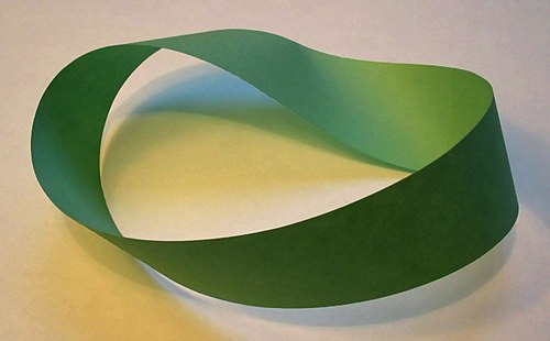
Great question. What even is a Mobius strip, anyways? Well, the image springs to mind of a long strip of paper, which has been twisted once, and then had its short ends joined. Here’s a picture, courtesy of Wikipedia:
So great, cool, a Mobius strip is a twisted piece of paper. But if you’re trying to visualize the process of cramming $g(L)$ onto that sheet of paper, you’re probably not having any fun. Our dimensionality doesn’t exactly add up in the same way.
Let’s focus on $g(L)$, but keep in mind our methods apply to $g(L_{\phi})$ as well .Is there a practical, tangible way to say that $g(L)$ is a Mobius strip? There is! The trick lies in “orientation.” An important feature of a Mobius strip is that, to creatures “living on the surface,” there is no notion of left-handed or right-handed. This is a very abstract concept, and Wikipedia once again provides a stellar example:
As you can see, the crab’s left claw is much larger than the right. It goes for a stroll, eventually returning to where it started, and then… Uh oh! At the end of the stroll, the crab’s right hand is now the larger one! This is very different from the reality you and I live in. A left-handed person won’t go for a walk and suddenly become right-handed.
Nevertheless, you can see the surface of a Mobius strip does not preserve orientation, so to speak. This is something we can visually identify in our data sets. Recall that in most of our animations, we “move through” $L$ or $L_{\phi}$ by sliding our two points on the original loop clockwise or counterclockwise. We have four “cardinal directions:” moving point 1 clockwise, moving point 1 counterclockwise, moving point 2 clockwise, and moving point 2 counterclockwise. We’ll call them North, South, East, and West respectively.
Here is an important claim about $L$ and $L_{\phi}$: at any point in $L$ or $L_{\phi}$, moving in a cardinal direction will always take you around the same loop. So say you’re standing at a point. You go for a stroll in a big loop. When you get back to where you started, North, South, East, and West all still point in the same direction. Orientation is preserved.
Now let’s talk about $g(L)$ and $g(L_{\phi})$. Is the same thing true? Not at all! You can go on a walk, end up back where you started, and suddenly West is South, North is East, and vice versa! The following visualization is a demonstration of this issue. Take a look, and then we’ll discuss it:
There are three steps in this animation
- Walk West until you end up where you started (we trace this)
- Walk in a special direction until you end up where you started
- Walk West until you end up where you started (compare to traced loop)
Here are the key points: in steps 1 and 3, we walk West from the same starting point, but we end up going different paths! In fact, the path we take in step 3 would have been the loop from going South in step 1! So what was the special direction in step 2? We walked in a loop around the twisted part of the mobius strip, just like the crab did in our previous example. This flipped our orientation around!
To see that each step was a loop, watch the graphs of $g(L)$. You’ll see it is always at the white points at the end and beginning of every loop. To drive this point home: this would never happen while walking around in $L$ or $L_{\phi}$. To those sets, North is North, and that’s the end of it. But since $(z,w)$ and $(w,z)$ take you to the same place in $g(L)$, we can swap the points of our input pair and flip our orientations around. That’s exactly what we did in step 2.
So we use the mapping $g$ to “ignore” the order of our pair of points, and as a result, it ends up being a mobius strip. We can observe this by noting that there are now loops that flip your orientation around. With this, we’re just about ready to tackle the final steps of this proof. We’re going to talk about “erasing” the trival intersections of $L$ and $L_{\phi}$ along $\lambda \times {0}$, and then we’re going to prove there are still some remaining intersections using these mobius strips.
Smoothing Out the Trivial Intersection
A Review and a Summary
Alright, here we are. The last big hurdle. We started with the question, “Given an arbitrary angle $\phi$ and a smooth Jordan curve $\lambda$, does there exist points on $\lambda$ which are the vertices of a rectangle with diagonal angle $\phi$?” We distilled this question slightly into “Are there two pairs of points on $\lambda$ which share the same midpoint, have the same pairwise distance, and have an angle $\phi$ between them?”
We distilled the question further into “Do the sets $L$ and $L_{\phi}$ have a nontrivial intersection? We distilled this yet again into “Do the sets $g(L)$ and $g(L_{\phi})$ have a nontrivial intersection?” At each step, we eliminated extra information, narrowing in on exactly the features that matter to our question.
Our next step is to eliminate the trivial intersections between $L$ and $L_{\phi}$, and thus between $g(L)$ and $g(L_{\phi})$ as well. What are the trivial intersections? $\lambda \times {0}$, as discussed previously. These pairs of points in $L$, $L_{\phi}$, etc all come from plugging in pairs on our loop of the form $(z,z)$. These points are useless information, and thus the intersection along $\lambda \times {0}$ is just distracting us.
The logic is like this: since $L$ and $L_{\phi}$ don’t self-intersect, we will try to remove their trivial intersection $\lambda \times {0}$ and smooth out the edges we’ve created so that all the structure is preserved. Then, instead of saying “Do $L$ and $L_{\phi}$ intersect nontrivially,” we will ask, “does the smoothed combination of $L$ and $L_{\phi}$ self-intersect?”
This is because now a self-intersection of the combination of $L$ and $L_{\phi}$ must be caused by a nontrivial intersection of $L$ and $L_{\phi}$, since we eliminated the trivial intersection in the smoothing process, and we know neither $L$ nor $L_{\phi}$ self-intersect individually.
So that’s where we’re at. We’re going to smooth out the trivial intersection, thus combining $L$ and $L_{\phi}$ into a single larger surface. We’ll engineer the smoothing so that the remaining combination ends up being a torus. But what is “smoothing?”
Starting at the End
What do we want when we smooth our trivial intersection? To answer this question, we’ll start exploring components of Propositions 1.1 and 1.2 in the original paper. At the end of the proof of Prop. 1.1, we see a summary of what our smoothing will look like:
\[\text {Replace }\left(L \cup L_{\phi}\right) \cap \mathcal{N}(\lambda) \text { by } \Psi\left(\left(S^{1} \times B \times\{0\}\right) \cap \mathcal{N}(\Gamma)\right)\]So we’re not supposed to understand all of this yet. Let’s look at the left side. $\mathcal{N}(\lambda)$ means “a neighborhood” around $\lambda$, or $\lambda\times{0}$ plus a little of the surrounding area. I think the authors mean $\lambda \times {0}$ here, but they left it out for efficiency.
So the first half of this makes sense. In our conjoined blob, $\left(L \cup L_{\phi}\right)$, we’re taking the points on this in a neighborhood of $\lambda \times {0}$ and swapping them out with something else. Now, the big question is, what is the “something else” here?
The right side of this equation uses a mathematical model the authors built which is equivalent to the neighborhood around $\lambda \times {0}$ in $\left(L \cup L_{\phi}\right)$. The model is much more tractable, so they solve the smoothing for the model. Then, they map this back to the actual intersection using $\Psi$. Let’s learn more about this model of the trivial intersection to understand how they did the smoothing.
A Local Model of the Trivial Intersection
Proposition 1.2 is the claim that the simple model space, $X$, contains a very boring curve, $\Gamma$, whose neighborhood, $\mathcal{N}(\Gamma)$, behaves identically to the neighborhood around our trivial intersection, $\mathcal{N}(\lambda)$. They have very simple surfaces, $L_0$ and $L_1$ in this model that intersect with $\Gamma$ just like $L$ and $L_{\phi}$ intersect with $\lambda \times {0}$
The four conditions express the properties of the model more clearly. The essence is that there exists a mapping which can take our boring, sterile model of the trivial intersection and bring it back to any real, messy, physical case. So all we need to do is describe the smoothing on our model, and then we’re done. But what is this model? Where was it constructed? This is the process of the proof of Proposition 1.2. But we’re about to hit a big road block, so let’s step back.
I’m Not Trained In Symplectic Geometry
Let’s start with the utility of symplectic math. All of the surfaces we have been working with are “symplectic manifolds,” and the Equivariant Darboux Theorem says (loosely) that all symplectic manifolds of the same dimension “look the same.” This is going to be useful for constructing our model of the area around the trivial intersection, but it doesn’t really answer any questions.
Unfortunately, I am not well-equipped to answer these questions. Here is a loose summary of where symplectic geometry fits into mathematics as a whole, and then we’ll sort of gloss over the details of these proofs.
Starting at the beginning, the topological properties of $\mathbb{R}$ enable us to perform calculus within the space. This is undisputably useful. However, historically people have had questions about shapes within the ambient space $\mathbb{R}^n$ (like a sphere, for example) that seemed to be complicated by the associated coordinates and such that come with the ambient space.
Since the surface of shapes like a sphere are “smooth” whether or not they’re embedded in $\mathbb{R}^n$, people began to reformulate calculus concepts so that they could be applied directly to shapes rather than to the ambient space, $\mathbb{R}^n$. This is smooth manifold theory, and it uses lots of topology and analysis.
To relate this to our current context, our starting curve $\lambda$ is a smooth manifold, and its cross product $\lambda \times \lambda$ is a smooth manifold, and most of our functions are homeomorphisms, meaning they map to other smooth manifolds with similar structure.
In fact, one of the big tools of smooth manifolds is mappings between different manifolds which preserve the properties you’re investigating. Different kinds of mappings preserve different properties of manifolds. A homeomorphism preserves less than a diffeomorphism. A diffeomorphism preserves less than a symplectomorphism. There are mappings that preserve more than a symplectomorphism or preserve different properties than a symplectomorphism.
Symplectomorphisms are the mappings we’re interested in here. In particular, a symplectomorphism preserves just the right amount of information so that we can make a model of the trivial intersection which is tractable. Then we can untangle the intersecting points with an “involution,” leaving only a smooth surface connecting $L$ and $L_{phi}$.
An Abrupt End
I believe I have stretched to my current limit in describing this paper. More than anything, I’m tired, and I don’t feel like exploring the local model right now. In the future, I may come and do a little walkthrough of the various components described. The meat of the construction occurs in Lemma 1.4, the summary of the local model is found just before Proposition 1.2, and the usage of the model appears in Proposition 1.2.
If anyone has actually read everything up to this point, I applaud your patience, and I’m deeply grateful for your participation in this little exercise. I hope to some day have the mathematical ability to finish this write-up in a satisfactory way. I’m optimistic my upcoming course in smooth manifolds will help me get closer to this goal.
More than anything, I hope this has made you feel that there is a way to “lift the veil” on abstract mathematics. It’s my deep conviction that mathematics is fundamentally and necessarily something which everyone has the capacity to understand. I think society stands to gain quite a bit from working not just on understanding new math, but also making the math we have more broadly comprehensible.
Je me casse!